Breadth-first search algorithm

Introduction

In Graph Theory 101, we introduced five concepts used to describe a graph: direction, weight, cycles, connectivity and density. In Modeling graphs using Python, we saw how to represent a graph using adjacency lists and adjacency matrices.

It is now time to learn how to traverse a connected graph. In this post, we introduce the breadth-first search algorithm (often shortened to BFS). We can run a BFS on either an adjacency list or an adjacency matrix.

What is breadth?

For the non-English speakers like me, let's look at a tree to better understand the notion of breadth.

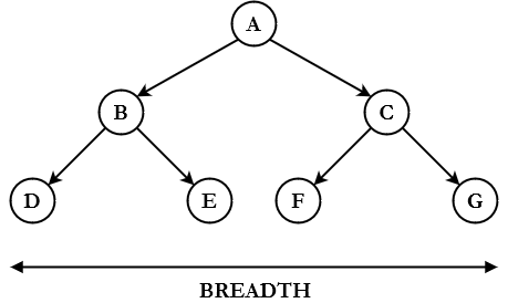
Remember that a tree is special type of graph, but breadth applies to all graphs.

Visual overview

Let's look at the below graph to understand how BFS works: from a given starting node, we list all the children. We then explore each child, and for each one of them, we list all its children. We then move another level down, etc.

In the above example, starting from A we list B and C. Moving to B, we list D and E. Moving to C, we list F and G. Moving to D, E, F and finally G, we realize they are leaf nodes so we don't list anything. When the list is empty, the algorithm stops.

Figure 1 is acyclic, but BFS needs to be able to explore cyclic graphs without getting trapped into infinite loops. To do so, we maintain a list of visited nodes and only add to the "next nodes" list unvisited ones.

In pseudo-code, the algorithm looks as follows:

function bfs(graph, node):
	visited = []
    

We will use the following unweighted directed graph as an example. It is slightly more complex than the ones we usually see in similar tutorials but it allows for a better understanding of how the algorithm works. As you can see

In a breadth-first search,

Python implementation

As discussed, we need to maintain two lists: a list of nodes that we already visited (in order to avoid infinite loops if the graph is cyclic) and a FIFO queue of nodes to visit.

For the list of visited nodes, we choose a set (since all elements will be unique) and for the FIFO queue of nodes to visit, we choose a deque, which is Python's queue data structure from the standard library.

Example of a bfs function printing all nodes:

AdjacencyList = dict[set]

def bfs(graph: AdjacencyList, node: int) -> None:
	visited = set()
    queue = deque()
    queue.append(node)

    while queue:
        node = queue.popleft()
        if node not in visited:
            visited.add(node)
            print(f"visiting node {node}:", end=" ")

            neighbors = graph[node]
            for neighbor in neighbors:
                if neighbor not in visited:
                    queue.append(neighbor)
                    print(f"{neighbor}", end=" ")

            print("")

Conclusion

What we do with BFS is very versatile: we can use BFS to explore all connected nodes, or to look for a specific node. We can use it to add edges etc.