Modeling graphs using Python

Introduction
In Graph Theory 101, we reviewed basic concepts from graph theory including direction, weight, cycles, connectivity and density. Be sure to read it first in order to be familiar with the vocabulary.
In this post, we discuss how to model nodes and edges using Python. Two data structures are commonly used in Computer Science to model graphs: adjacency matrices and adjacency lists. Both structures can be used to represent any type of graph, but they come with specific trade-offs.
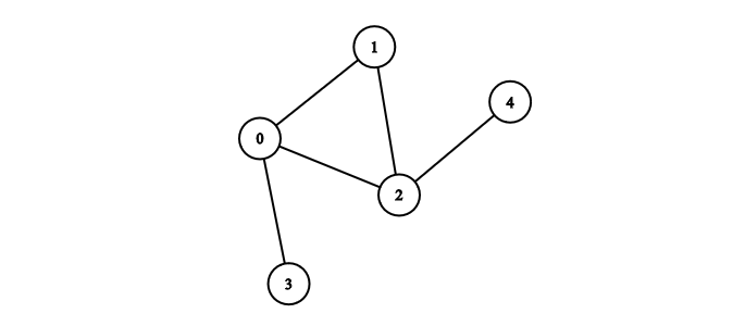
Below is the graph we will use throughout the article. It is unweighted, undirected, connected and neither really sparse nor dense.
The adjacency matrix
Definition
An adjacency matrix is a square matrix where matrix[i][j] represents the cost of moving from node i to node j.
If the graph is unweighted, we assume the default cost to be 1. So if nodes i and j are connected, matrix[i][j] = 1, otherwise matrix[i][j] = 0. If the graph is weighted, matrix[i][j] contains the edge's weight.
If the graph is undirected, i.e. all edges are bi-directional, the matrix is symmetric: each entry is equal to its transpose.
| graph type | matrix characteristics |
|---|---|
| unweighted | filled with 0s and 1s |
| weighted | filled with 0s and weights |
| undirected | symmetric |
| directed | not symmetric |
Complexity
Assuming the graph has \(n\) nodes: the space complexity of storing the matrix is \(O(n^2)\) as we need memory for all possible edges, but the time complexity of querying for an edge is only \(O(1)\) since we can directly look it up.
Python implementation
In Python, we can model the adjacency matrix using a list of lists or a list of dictionaries.
In the most simple case, we label the nodes as a list of integers starting at zero. We can then use a Python list of lists to model the adjacency matrix, where each index of the list is also a node.
We can build the adjacency matrix for Figure 1 from a list of edges as follows:
# Inputs
nodes = [0, 1, 2, 3, 4]
edges = [[0, 1], [0, 2], [1, 2], [3, 0], [4, 2]]

# Adjacency matrix
graph = [[0 for i in range(5)] for j in range(5)]
for edge in edges:
    graph[edge[0]][edge[1]] = 1
    graph[edge[1]][edge[0]] = 1
Result:
>>> graph
[[0, 1, 1, 1, 0],
 [1, 0, 1, 0, 0],
 [1, 1, 0, 0, 1],
 [1, 0, 0, 0, 0],
 [0, 0, 1, 0, 0]]
To check if there is an edge between nodes 1 and 2 we simply lookup the value of graph[1][2].
The adjacency list
Definition
An adjacency list only represents existing edges. It is a list of lists where each first list represents a node and each second list is the list of neighboring nodes.
Complexity
Assuming the graph has \(n\) nodes and \(m\) edges, the space complexity of storing the adjacency list is \(O(m + n)\) since we only store existing edges, but the time complexity of finding an edge is \(O(n)\) since, for a given node, we need to loop through all the neighbors to see whether the edge exists.
Python implementation
Using the same example as before, we can implement the adjacency list in Python using a dictionary of sets:
# Inputs
nodes = [0, 1, 2, 3, 4]
edges = [[0, 1], [0, 2], [1, 2], [3, 0], [4, 2]]

# Adjacency list
graph = defaultdict(set)
for edge in edges:
    graph[edge[0]].add(edge[1])
    graph[edge[1]].add(edge[0])
Result:
>>> graph
defaultdict(<class 'set'>,
	{
		0: {1, 2, 3},
		1: {0, 2},
		2: {0, 1, 4},
		3: {0},
		4: {2}
	}
)
In order to see whether there is an edge between nodes 1 and 2, we either loop through graph[1] in search of 2 or loop through graph[2] in search of 1.
Conclusion
In this post we reviewed both adjacency matrices and adjacency lists. Adjacency matrices are best suited for dense graphs whereas adjacency lists are more efficient for sparse graphs.
In the next post, we will look at how to traverse a graph using breadth-first search algorithm.
Although useful for general understanding (and for programming interviews!), it is recommended not to reinvent the wheel in production code. Instead, it is better to use existing libraries such as networkx to model and analyze graphs.
References: